Note
Click here to download the full example code
Tree LSTM DGL Tutorial
Author: Zihao Ye, Qipeng Guo, Minjie Wang, Jake Zhao, Zheng Zhang
Tree-LSTM structure was first introduced by Kai et. al in an ACL 2015 paper: Improved Semantic Representations From Tree-Structured Long Short-Term Memory Networks. The core idea is to introduce syntactic information for language tasks by extending the chain-structured LSTM to a tree-structured LSTM. The Dependency Tree/Constituency Tree techniques were leveraged to obtain a ‘’latent tree’‘.
One, if not all, difficulty of training Tree-LSTMs is batching — a standard technique in machine learning to accelerate optimization. However, since trees generally have different shapes by nature, parallization becomes non trivial. DGL offers an alternative: to pool all the trees into one single graph then induce the message passing over them guided by the structure of each tree.
The task and the dataset
In this tutorial, we will use Tree-LSTMs for sentiment analysis.
We have wrapped the
Stanford Sentiment Treebank in
dgl.data. The dataset provides a fine-grained tree level sentiment
annotation: 5 classes(very negative, negative, neutral, positive, and
very positive) that indicates the sentiment in current subtree. Non-leaf
nodes in constituency tree does not contain words, we use a special
PAD_WORD token to denote them, during the training/inferencing,
their embeddings would be masked to all-zero.
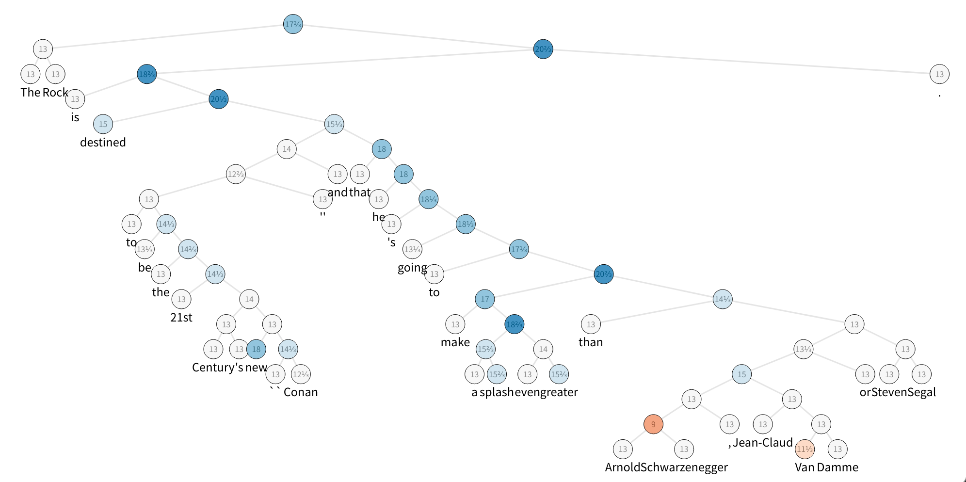
The figure displays one sample of the SST dataset, which is a constituency parse tree with their nodes labeled with sentiment. To speed up things, let’s build a tiny set with 5 sentences and take a look at the first one:
import dgl
from dgl.data.tree import SST
from dgl.data import SSTBatch

# Each sample in the dataset is a constituency tree. The leaf nodes
# represent words. The word is a int value stored in the "x" field.
# The non-leaf nodes has a special word PAD_WORD. The sentiment
# label is stored in the "y" feature field.
trainset = SST(mode='tiny')  # the "tiny" set has only 5 trees
tiny_sst = trainset.trees
num_vocabs = trainset.num_vocabs
num_classes = trainset.num_classes

vocab = trainset.vocab # vocabulary dict: key -> id
inv_vocab = {v: k for k, v in vocab.items()} # inverted vocabulary dict: id -> word

a_tree = tiny_sst[0]
for token in a_tree.ndata['x'].tolist():
    if token != trainset.PAD_WORD:
        print(inv_vocab[token], end=" ")
Out:
Preprocessing...
Dataset creation finished. #Trees: 5
the rock is destined to be the 21st century 's new `` conan '' and that he 's going to make a splash even greater than arnold schwarzenegger , jean-claud van damme or steven segal .
Step 1: batching
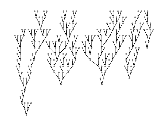
The first step is to throw all the trees into one graph, using
the batch() API.
import networkx as nx
import matplotlib.pyplot as plt

graph = dgl.batch(tiny_sst)
def plot_tree(g):
    # this plot requires pygraphviz package
    pos = nx.nx_agraph.graphviz_layout(g, prog='dot')
    nx.draw(g, pos, with_labels=False, node_size=10,
            node_color=[[.5, .5, .5]], arrowsize=4)
    plt.show()

plot_tree(graph.to_networkx())
You can read more about the definition of batch()
(by clicking the API), or can skip ahead to the next step:
Note
Definition: a BatchedDGLGraph is a
DGLGraph that unions a list of DGLGraphs.
The union includes all the nodes, edges, and their features. The order of nodes, edges and features are preserved.
- Given that we have \(V_i\) nodes for graph \(\mathcal{G}_i\), the node ID \(j\) in graph \(\mathcal{G}_i\) correspond to node ID \(j + \sum_{k=1}^{i-1} V_k\) in the batched graph.
- Therefore, performing feature transformation and message passing on
BatchedDGLGraphis equivalent to doing those on allDGLGraphconstituents in parallel.
Duplicate references to the same graph are treated as deep copies; the nodes, edges, and features are duplicated, and mutation on one reference does not affect the other.
Currently,
BatchedDGLGraphis immutable in graph structure (i.e. one can’t add nodes and edges to it). We need to support mutable batched graphs in (far) future.The
BatchedDGLGraphkeeps track of the meta information of the constituents so it can beunbatch()ed to list ofDGLGraphs.
For more details about the BatchedDGLGraph
module in DGL, you can click the class name.
Step 2: Tree-LSTM Cell with message-passing APIs
The authors proposed two types of Tree LSTM: Child-Sum Tree-LSTMs, and \(N\)-ary Tree-LSTMs. In this tutorial we focus on applying Binary Tree-LSTM to binarized constituency trees(this application is also known as Constituency Tree-LSTM). We use PyTorch as our backend framework to set up the network.
In N-ary Tree LSTM, each unit at node \(j\) maintains a hidden representation \(h_j\) and a memory cell \(c_j\). The unit \(j\) takes the input vector \(x_j\) and the hidden representations of the their child units: \(h_{jl}, 1\leq l\leq N\) as input, then update its new hidden representation \(h_j\) and memory cell \(c_j\) by:
It can be decomposed into three phases: message_func,
reduce_func and apply_node_func.
Note
apply_node_func is a new node UDF we have not introduced before. In
apply_node_func, user specifies what to do with node features,
without considering edge features and messages. In Tree-LSTM case,
apply_node_func is a must, since there exists (leaf) nodes with
\(0\) incoming edges, which would not be updated via
reduce_func.
import torch as th
import torch.nn as nn

class TreeLSTMCell(nn.Module):
    def __init__(self, x_size, h_size):
        super(TreeLSTMCell, self).__init__()
        self.W_iou = nn.Linear(x_size, 3 * h_size, bias=False)
        self.U_iou = nn.Linear(2 * h_size, 3 * h_size, bias=False)
        self.b_iou = nn.Parameter(th.zeros(1, 3 * h_size))
        self.U_f = nn.Linear(2 * h_size, 2 * h_size)

    def message_func(self, edges):
        return {'h': edges.src['h'], 'c': edges.src['c']}

    def reduce_func(self, nodes):
        # concatenate h_jl for equation (1), (2), (3), (4)
        h_cat = nodes.mailbox['h'].view(nodes.mailbox['h'].size(0), -1)
        # equation (2)
        f = th.sigmoid(self.U_f(h_cat)).view(*nodes.mailbox['h'].size())
        # second term of equation (5)
        c = th.sum(f * nodes.mailbox['c'], 1)
        return {'iou': self.U_iou(h_cat), 'c': c}

    def apply_node_func(self, nodes):
        # equation (1), (3), (4)
        iou = nodes.data['iou'] + self.b_iou
        i, o, u = th.chunk(iou, 3, 1)
        i, o, u = th.sigmoid(i), th.sigmoid(o), th.tanh(u)
        # equation (5)
        c = i * u + nodes.data['c']
        # equation (6)
        h = o * th.tanh(c)
        return {'h' : h, 'c' : c}
Step 3: define traversal
After defining the message passing functions, we then need to induce the right order to trigger them. This is a significant departure from models such as GCN, where all nodes are pulling messages from upstream ones simultaneously.
In the case of Tree-LSTM, messages start from leaves of the tree, and propagate/processed upwards until they reach the roots. A visualization is as follows:
DGL defines a generator to perform the topological sort, each item is a tensor recording the nodes from bottom level to the roots. One can appreciate the degree of parallelism by inspecting the difference of the followings:
print('Traversing one tree:')
print(dgl.topological_nodes_generator(a_tree))

print('Traversing many trees at the same time:')
print(dgl.topological_nodes_generator(graph))
Out:
Traversing one tree:
(tensor([ 2,  3,  6,  8, 13, 15, 17, 19, 22, 23, 25, 27, 28, 29, 30, 32, 34, 36,
        38, 40, 43, 46, 47, 49, 50, 52, 58, 59, 60, 62, 64, 65, 66, 68, 69, 70]), tensor([ 1, 21, 26, 45, 48, 57, 63, 67]), tensor([24, 44, 56, 61]), tensor([20, 42, 55]), tensor([18, 54]), tensor([16, 53]), tensor([14, 51]), tensor([12, 41]), tensor([11, 39]), tensor([10, 37]), tensor([35]), tensor([33]), tensor([31]), tensor([9]), tensor([7]), tensor([5]), tensor([4]), tensor([0]))
Traversing many trees at the same time:
(tensor([  2,   3,   6,   8,  13,  15,  17,  19,  22,  23,  25,  27,  28,  29,
         30,  32,  34,  36,  38,  40,  43,  46,  47,  49,  50,  52,  58,  59,
         60,  62,  64,  65,  66,  68,  69,  70,  74,  76,  78,  79,  82,  83,
         85,  88,  90,  92,  93,  95,  96, 100, 102, 103, 105, 109, 110, 112,
        113, 117, 118, 119, 121, 125, 127, 129, 130, 132, 133, 135, 138, 140,
        141, 142, 143, 150, 152, 153, 155, 158, 159, 161, 162, 164, 168, 170,
        171, 174, 175, 178, 179, 182, 184, 185, 187, 189, 190, 191, 192, 195,
        197, 198, 200, 202, 205, 208, 210, 212, 213, 214, 216, 218, 219, 220,
        223, 225, 227, 229, 230, 232, 235, 237, 240, 242, 244, 246, 248, 249,
        251, 253, 255, 256, 257, 259, 262, 263, 267, 269, 270, 271, 272]), tensor([  1,  21,  26,  45,  48,  57,  63,  67,  77,  81,  91,  94, 101, 108,
        111, 116, 128, 131, 139, 151, 157, 160, 169, 173, 177, 183, 188, 196,
        211, 217, 228, 247, 254, 261, 268]), tensor([ 24,  44,  56,  61,  75,  89,  99, 107, 115, 126, 137, 149, 156, 167,
        181, 186, 194, 209, 215, 226, 245, 252, 266]), tensor([ 20,  42,  55,  73,  87, 124, 136, 154, 180, 207, 224, 243, 250, 265]), tensor([ 18,  54,  86, 123, 134, 148, 176, 206, 222, 241, 264]), tensor([ 16,  53,  84, 122, 172, 204, 239, 260]), tensor([ 14,  51,  80, 120, 166, 203, 238, 258]), tensor([ 12,  41,  72, 114, 165, 201, 236]), tensor([ 11,  39, 106, 163, 199, 234]), tensor([ 10,  37, 104, 147, 193, 233]), tensor([ 35,  98, 146, 231]), tensor([ 33,  97, 145, 221]), tensor([ 31,  71, 144]), tensor([9]), tensor([7]), tensor([5]), tensor([4]), tensor([0]))
We then call prop_nodes() to trigger the message passing:
import dgl.function as fn
import torch as th

graph.ndata['a'] = th.ones(graph.number_of_nodes(), 1)
graph.register_message_func(fn.copy_src('a', 'a'))
graph.register_reduce_func(fn.sum('a', 'a'))

traversal_order = dgl.topological_nodes_generator(graph)
graph.prop_nodes(traversal_order)

# the following is a syntax sugar that does the same
# dgl.prop_nodes_topo(graph)
Note
Before we call prop_nodes(), we must specify a
message_func and reduce_func in advance, here we use built-in
copy-from-source and sum function as our message function and reduce
function for demonstration.
Putting it together
Here is the complete code that specifies the Tree-LSTM class:
class TreeLSTM(nn.Module):
    def __init__(self,
                 num_vocabs,
                 x_size,
                 h_size,
                 num_classes,
                 dropout,
                 pretrained_emb=None):
        super(TreeLSTM, self).__init__()
        self.x_size = x_size
        self.embedding = nn.Embedding(num_vocabs, x_size)
        if pretrained_emb is not None:
            print('Using glove')
            self.embedding.weight.data.copy_(pretrained_emb)
            self.embedding.weight.requires_grad = True
        self.dropout = nn.Dropout(dropout)
        self.linear = nn.Linear(h_size, num_classes)
        self.cell = TreeLSTMCell(x_size, h_size)

    def forward(self, batch, h, c):
        """Compute tree-lstm prediction given a batch.

        Parameters
        ----------
        batch : dgl.data.SSTBatch
            The data batch.
        h : Tensor
            Initial hidden state.
        c : Tensor
            Initial cell state.

        Returns
        -------
        logits : Tensor
            The prediction of each node.
        """
        g = batch.graph
        g.register_message_func(self.cell.message_func)
        g.register_reduce_func(self.cell.reduce_func)
        g.register_apply_node_func(self.cell.apply_node_func)
        # feed embedding
        embeds = self.embedding(batch.wordid * batch.mask)
        g.ndata['iou'] = self.cell.W_iou(self.dropout(embeds)) * batch.mask.float().unsqueeze(-1)
        g.ndata['h'] = h
        g.ndata['c'] = c
        # propagate
        dgl.prop_nodes_topo(g)
        # compute logits
        h = self.dropout(g.ndata.pop('h'))
        logits = self.linear(h)
        return logits
Main Loop
Finally, we could write a training paradigm in PyTorch:
from torch.utils.data import DataLoader
import torch.nn.functional as F

device = th.device('cpu')
# hyper parameters
x_size = 256
h_size = 256
dropout = 0.5
lr = 0.05
weight_decay = 1e-4
epochs = 10

# create the model
model = TreeLSTM(trainset.num_vocabs,
                 x_size,
                 h_size,
                 trainset.num_classes,
                 dropout)
print(model)

# create the optimizer
optimizer = th.optim.Adagrad(model.parameters(),
                          lr=lr,
                          weight_decay=weight_decay)

def batcher(dev):
    def batcher_dev(batch):
        batch_trees = dgl.batch(batch)
        return SSTBatch(graph=batch_trees,
                        mask=batch_trees.ndata['mask'].to(device),
                        wordid=batch_trees.ndata['x'].to(device),
                        label=batch_trees.ndata['y'].to(device))
    return batcher_dev

train_loader = DataLoader(dataset=tiny_sst,
                          batch_size=5,
                          collate_fn=batcher(device),
                          shuffle=False,
                          num_workers=0)

# training loop
for epoch in range(epochs):
    for step, batch in enumerate(train_loader):
        g = batch.graph
        n = g.number_of_nodes()
        h = th.zeros((n, h_size))
        c = th.zeros((n, h_size))
        logits = model(batch, h, c)
        logp = F.log_softmax(logits, 1)
        loss = F.nll_loss(logp, batch.label, reduction='sum')
        optimizer.zero_grad()
        loss.backward()
        optimizer.step()
        pred = th.argmax(logits, 1)
        acc = float(th.sum(th.eq(batch.label, pred))) / len(batch.label)
        print("Epoch {:05d} | Step {:05d} | Loss {:.4f} | Acc {:.4f} |".format(
            epoch, step, loss.item(), acc))
Out:
TreeLSTM(
  (embedding): Embedding(19536, 256)
  (dropout): Dropout(p=0.5)
  (linear): Linear(in_features=256, out_features=5, bias=True)
  (cell): TreeLSTMCell(
    (W_iou): Linear(in_features=256, out_features=768, bias=False)
    (U_iou): Linear(in_features=512, out_features=768, bias=False)
    (U_f): Linear(in_features=512, out_features=512, bias=True)
  )
)
Epoch 00000 | Step 00000 | Loss 448.3144 | Acc 0.1575 |
Epoch 00001 | Step 00000 | Loss 251.1886 | Acc 0.7582 |
Epoch 00002 | Step 00000 | Loss 241.3439 | Acc 0.7326 |
Epoch 00003 | Step 00000 | Loss 400.2593 | Acc 0.8132 |
Epoch 00004 | Step 00000 | Loss 579.3557 | Acc 0.6154 |
Epoch 00005 | Step 00000 | Loss 167.4419 | Acc 0.8498 |
Epoch 00006 | Step 00000 | Loss 94.3875 | Acc 0.8938 |
Epoch 00007 | Step 00000 | Loss 82.4258 | Acc 0.9048 |
Epoch 00008 | Step 00000 | Loss 77.3624 | Acc 0.9048 |
Epoch 00009 | Step 00000 | Loss 68.1858 | Acc 0.9121 |
To train the model on full dataset with different settings(CPU/GPU, etc.), please refer to our repo’s example. Besides, we also provide an implementation of the Child-Sum Tree LSTM.
Total running time of the script: ( 0 minutes 1.275 seconds)