Hypergraph Neural Networks
This tutorial illustrates what is hypergraph and how to build a Hypergraph Neural Network using DGL’s sparse matrix APIs.
![]()
[ ]:
# Install required packages.
import os
import torch
os.environ['TORCH'] = torch.__version__
os.environ['DGLBACKEND'] = "pytorch"

# Uncomment below to install required packages. If the CUDA version is not 11.8,
# check the https://www.dgl.ai/pages/start.html to find the supported CUDA
# version and corresponding command to install DGL.
#!pip install dgl -f https://data.dgl.ai/wheels/cu118/repo.html > /dev/null
#!pip install torchmetrics > /dev/null

try:
    import dgl
    installed = True
except ImportError:
    installed = False
print("DGL installed!" if installed else "Failed to install DGL!")
Hypergraphs
A hypergraph consists of nodes and hyperedges. Contrary to edges in graphs, a hyperedge can connect arbitrary number of nodes. For instance, the following figure shows a hypergraph with 11 nodes and 5 hyperedges drawn in different colors. 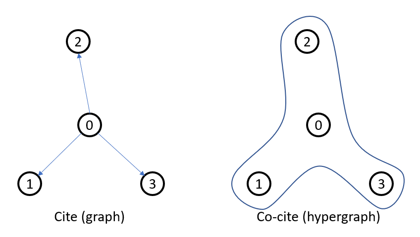
Hypergraphs are particularly useful when the relationships between data points within the dataset is not binary. For instance, more than two products can be co-purchased together in an e-commerce system, so the relationship of co-purchase is \(n\)-ary rather than binary, and therefore it is better described as a hypergraph rather than a normal graph.
A hypergraph is usually characterized by its incidence matrix \(H\), whose rows represent nodes and columns represent hyperedges. An entry \(H_{ij}\) is 1 if hyperedge \(j\) includes node \(i\), or 0 otherwise. For example, the hypergraph in the figure above can be characterized by a \(11 \times 5\) matrix as follows:
One can construct the hypergraph incidence matrix by specifying two tensors nodes and hyperedges, where the node ID nodes[i] belongs to the hyperedge ID hyperedges[i] for all i. In the case above, the incidence matrix can be constructed below.
[ ]:
import dgl.sparse as dglsp
import torch

H = dglsp.spmatrix(
    torch.LongTensor([[0, 1, 2, 2, 2, 2, 3, 4, 5, 5, 5, 5, 6, 7, 7, 8, 8, 9, 9, 10],
                      [0, 0, 0, 1, 3, 4, 2, 1, 0, 2, 3, 4, 2, 1, 3, 1, 3, 2, 4, 4]])
)

print(H.to_dense())
tensor([[1., 0., 0., 0., 0.],
        [1., 0., 0., 0., 0.],
        [1., 1., 0., 1., 1.],
        [0., 0., 1., 0., 0.],
        [0., 1., 0., 0., 0.],
        [1., 0., 1., 1., 1.],
        [0., 0., 1., 0., 0.],
        [0., 1., 0., 1., 0.],
        [0., 1., 0., 1., 0.],
        [0., 0., 1., 0., 1.],
        [0., 0., 0., 0., 1.]])
The degree of a node in a hypergraph is defined as the number of hyperedges including the node. Similarly, the degree of a hyperedge in a hypergraph is defined as the number of nodes included by the hyperedge. In the example above, the hyperedge degrees can be computed by the sum of row vectors (i.e. all 4), while the node degree can be computed by the sum of column vectors.
[ ]:
node_degrees = H.sum(1)
print("Node degrees", node_degrees)

hyperedge_degrees = H.sum(0)
print("Hyperedge degrees", hyperedge_degrees)
Node degrees tensor([1., 1., 4., 1., 1., 4., 1., 2., 2., 2., 1.])
Hyperedge degrees tensor([4., 4., 4., 4., 4.])
Hypergraph Neural Network (HGNN) Layer
The HGNN layer is defined as:
where
\(H \in \mathbb{R}^{N \times M}\) is the incidence matrix of hypergraph with \(N\) nodes and \(M\) hyperedges.
\(D_v \in \mathbb{R}^{N \times N}\) is a diagonal matrix representing node degrees, whose \(i\)-th diagonal element is \(\sum_{j=1}^M H_{ij}\).
\(D_e \in \mathbb{R}^{M \times M}\) is a diagonal matrix representing hyperedge degrees, whose \(j\)-th diagonal element is \(\sum_{i=1}^N H_{ij}\).
\(B \in \mathbb{R}^{M \times M}\) is a diagonal matrix representing the hyperedge weights, whose \(j\)-th diagonal element is the weight of \(j\)-th hyperedge. In our example, \(B\) is an identity matrix.
The following code builds a two-layer HGNN.
[ ]:
import dgl.sparse as dglsp
import torch
import torch.nn as nn
import torch.nn.functional as F
import tqdm
from dgl.data import CoraGraphDataset
from torchmetrics.functional import accuracy


class HGNN(nn.Module):
    def __init__(self, H, in_size, out_size, hidden_dims=16):
        super().__init__()

        self.W1 = nn.Linear(in_size, hidden_dims)
        self.W2 = nn.Linear(hidden_dims, out_size)
        self.dropout = nn.Dropout(0.5)

        ###########################################################
        # (HIGHLIGHT) Compute the Laplacian with Sparse Matrix API
        ###########################################################
        # Compute node degree.
        d_V = H.sum(1)
        # Compute edge degree.
        d_E = H.sum(0)
        # Compute the inverse of the square root of the diagonal D_v.
        D_v_invsqrt = dglsp.diag(d_V**-0.5)
        # Compute the inverse of the diagonal D_e.
        D_e_inv = dglsp.diag(d_E**-1)
        # In our example, B is an identity matrix.
        n_edges = d_E.shape[0]
        B = dglsp.identity((n_edges, n_edges))
        # Compute Laplacian from the equation above.
        self.L = D_v_invsqrt @ H @ B @ D_e_inv @ H.T @ D_v_invsqrt

    def forward(self, X):
        X = self.L @ self.W1(self.dropout(X))
        X = F.relu(X)
        X = self.L @ self.W2(self.dropout(X))
        return X
Loading Data
We use Cora citation network in our example. But instead of using the original “cite” relationship between papers, we consider the “co-cite” relationship between papers. We build a hypergraph from the original citation network where for each paper we construct a hyperedge that includes all the other papers it cited, as well as the paper itself.
Note that a hypergraph constructed this way has an incidence matrix exactly identical to the adjacency matrix of the original graph (plus an identity matrix for self-loops). This is because each hyperedge has a one-to-one correspondence to each paper. So we can directly take the graph’s adjacency matrix and add an identity matrix to it, and we use it as the hypergraph’s incidence matrix.
[ ]:
def load_data():
    dataset = CoraGraphDataset()

    graph = dataset[0]
    indices = torch.stack(graph.edges())
    H = dglsp.spmatrix(indices)
    H = H + dglsp.identity(H.shape)

    X = graph.ndata["feat"]
    Y = graph.ndata["label"]
    train_mask = graph.ndata["train_mask"]
    val_mask = graph.ndata["val_mask"]
    test_mask = graph.ndata["test_mask"]
    return H, X, Y, dataset.num_classes, train_mask, val_mask, test_mask
Training and Evaluation
Now we can write the training and evaluation functions as follows.
[ ]:
def train(model, optimizer, X, Y, train_mask):
    model.train()
    Y_hat = model(X)
    loss = F.cross_entropy(Y_hat[train_mask], Y[train_mask])
    optimizer.zero_grad()
    loss.backward()
    optimizer.step()


def evaluate(model, X, Y, val_mask, test_mask, num_classes):
    model.eval()
    Y_hat = model(X)
    val_acc = accuracy(
        Y_hat[val_mask], Y[val_mask], task="multiclass", num_classes=num_classes
    )
    test_acc = accuracy(
        Y_hat[test_mask],
        Y[test_mask],
        task="multiclass",
        num_classes=num_classes,
    )
    return val_acc, test_acc


H, X, Y, num_classes, train_mask, val_mask, test_mask = load_data()
model = HGNN(H, X.shape[1], num_classes)
optimizer = torch.optim.Adam(model.parameters(), lr=0.001)

with tqdm.trange(500) as tq:
    for epoch in tq:
        train(model, optimizer, X, Y, train_mask)
        val_acc, test_acc = evaluate(
            model, X, Y, val_mask, test_mask, num_classes
        )
        tq.set_postfix(
            {
                "Val acc": f"{val_acc:.5f}",
                "Test acc": f"{test_acc:.5f}",
            },
            refresh=False,
        )

print(f"Test acc: {test_acc:.3f}")
Downloading /root/.dgl/cora_v2.zip from https://data.dgl.ai/dataset/cora_v2.zip...
Extracting file to /root/.dgl/cora_v2
Finished data loading and preprocessing.
  NumNodes: 2708
  NumEdges: 10556
  NumFeats: 1433
  NumClasses: 7
  NumTrainingSamples: 140
  NumValidationSamples: 500
  NumTestSamples: 1000
Done saving data into cached files.
100%|██████████| 500/500 [00:57<00:00, 8.70it/s, Val acc=0.77800, Test acc=0.78100]
Test acc: 0.781
For the complete example of HGNN, please refer to here.